
Anna Peters, Richard Peters
Peters Research Ltd
This paper was presented at The 10th Symposium on Lift & Escalator Technology (CIBSE Lifts Group, The University of Northampton and LEIA) (2019). This web version © Peters Research Ltd 2019
Keywords: Kinematics, accelerometer, performance, logging, passenger demand
Abstract. Data measured with an accelerometer in or on a lift car can be very useful. Using an accelerometer to measure individual trips allows engineers to confirm that a lift is working as specified. Further analysis of extended measurements can also provide an understanding of lift passenger demand, useful in planning new buildings and addressing traffic problems in existing buildings. Accelerometers can also be used as part of lift monitoring systems, collecting data about the lifts without the need for interfacing with lift controllers, which can be expensive due to the use of proprietary protocols. In this paper the authors address the analysis of accelerometer data for a multi trip scenario. With real as opposed to ideal data, the analysis procedure must account for accelerometer drift, noise and other data anomalies. The final analysis software provides an idealised version of the measured data including the distance, velocity, acceleration and jerk for each trip. The distance measurements combined provide a spatial plot of lift position.
1 Introduction
The logging of lift motion is valuable when measuring lift performance, analysing lift traffic and lift monitoring. Accelerometers can be used as part of lift monitoring systems, collecting data without the need for interfacing with lift controllers, which can be expensive due to the use of proprietary protocols [1].
Software has been developed to process data collected by a low-cost computer and accelerometer placed on top of a lift car. By analysing a sequence of individual lift journeys, the software is able to provide a summary of lift stops analysed by floor and time of day.
1.1 Motivation
Estimates of lift passenger demand are required in the planning of new lift installations and when addressing lift traffic problems in existing buildings. By recording and processing the output of an accelerometer, a spatial plot of lift motion can be produced. An indication of lift passenger demand can then be determined without the need for human observers.
This is possible as the spatial plot data recorded by the accelerometer software can be applied in the development of mathematical models to extrapolate passenger demand from stops. This work is outside the scope of this paper, but a range of methods have been proposed by several researchers over many years [2], [3] with recent work showing how good passenger demand predictions can be estimated with limited data sets [4].
The software developed can also support the monitoring of lift installations by providing a connection-free solution. Because the application of interfacing standards is rare, third party monitoring of lift installations can be expensive.
1.2 Ideal Lift Kinematics
It is possible to derive equations to represent the ideal motion of a lift, which can be plotted as continuous functions that represent the optimum displacement (D), velocity (V), acceleration (A) and jerk (J) profiles, see Figure 1.
Modern variable speed drives can be programmed to match these ideal lift kinematics curves closely. Since it is necessary to model each lift trip as accurately as possible, a good approach is to fit the measured accelerometer data to the idealised kinematics plots.
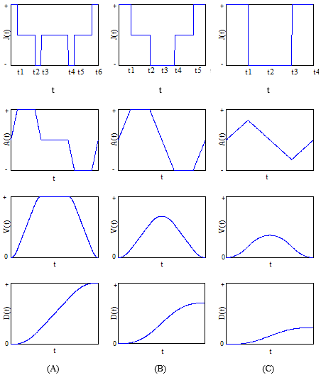
Figure 1 [5]: Ideal lift kinematics for: (A) lift reaches full speed; (B) lift reaches full acceleration, but not full speed; (C) lift does not reach full speed or acceleration
Ideal lift kinematics represents a lift acceleration profile by a series of straight lines. The software therefore applies a linear regression method to fit raw measured data to an ideal plot.
2 Coding methodology
2.1 Raw Accelerometer Data
The software is required to process a full set of raw accelerometer data as shown in Figure 2.
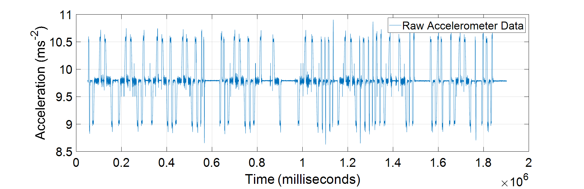
Figure 2: Multiple Lift Trip Raw Accelerometer Plot
To simplify the problem, the data set is isolated into a series of single up and down lift journeys (trips) that can each be analysed individually. An example of an isolated single trip is illustrated in Figure 3.
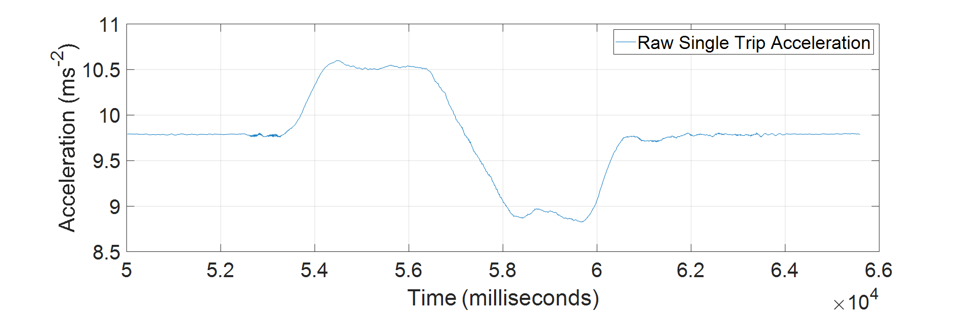
Figure 3: Single Lift Trip Raw Accelerometer Plot
2.2 Language Selection
The software was written in the C++ programming language and is object orientated. Object orientated programming combines groups of related variables and functions into a class. Properties and methods can be hidden inside the class making the software easier to use, understand and maintain [6].
2.3 Processing Ideal Data
The basic methodology of the software was created, and initially tested on self-generated ideal lift journeys. This ensured that the code could correctly follow an expected journey before tackling real world data. These ideal journeys followed a profile identical to ideal lift kinematics curves, therefore the software outputted an identical profile.
Each isolated single trip can be separated into two phases, one of acceleration and the other deceleration. Since it is assumed that the accelerometer data will start and finish with a stationary lift, there will be an even number of acceleration and deceleration phases. Therefore, for each single trip, the following analysis is carried out twice, once for each phase.
It must be decided whether another phase exists. A new phase occurs when the modulus of the acceleration reaches a threshold value, 50% of the maximum acceleration identified. The next phase is the first case in the remaining data set that this threshold is reached, as shown in Figure 4.
If a phase is identified, it must be determined whether this is an acceleration or deceleration phase. A positive acceleration determines an acceleration phase and a negative value determines a deceleration phase.
For each phase, linear regression analysis is carried out on the two sections where acceleration is non-constant:
(a) Modulus of the acceleration rising
(b) Modulus of the acceleration falling
In anticipation of noise that will be present in real data, linear regression analysis is not carried out over the full length of the phase sections. A reasonable assumption is to carry out analysis on the segments of the sections that fall within 20% and 60% of the maximum acceleration.
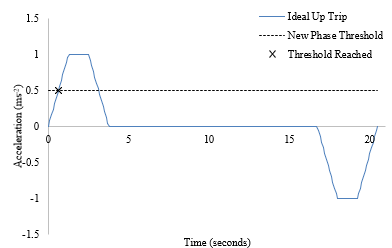
Figure 4: Identification of an Acceleration Phase Within an Up Trip
Linear regression analysis is carried out on all the data that falls between the four calculated limits. Two linear regression lines are identified that minimise the sum of the squares of the errors between the lines and the raw data, with results shown in Figure 5.
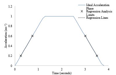
Figure 5: Linear Regression Fit of Acceleration Profile Between Calculated Limits
The software identifies the length of the regression lines (that are to be joined with a horizontal line in specific cases) that minimise the sum of the squares of the errors between the approximated and the raw accelerometer data. Figure 6 demonstrates the process of extending the regression line to the length of minimum error.
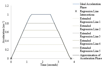
Figure 6: Identification of the Correct Regression Line Length
The series of time and acceleration coordinates to represent each phase are stored in a vector. Zero acceleration coordinates are added from the start of the test data to the beginning of the acceleration/deceleration phase. The regression analysis is then repeated for the second phase of the trip. Figure 7 plots the approximated single up trip profile against the ideal up trip, confirming that the software could accurately represent the data prior to testing on real data.
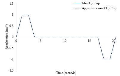
Figure 7: Ideal vs. Approximated Acceleration Profiles of a Single Up Trip
An approximation of the ideal jerk profile is generated via a central difference differentiation of the approximated acceleration profile.
A trapezium rule integration is carried out on the approximated acceleration profile, generating an approximated velocity profile. From ideal lift kinematics, it is known that the integral of a single trip should equal zero, since the lift starts and ends stationary. A scaling factor is determined from the difference between the integrals of the acceleration and deceleration phases. This scaling factor is applied to the acceleration profile such that the integral will equal zero.
To determine the approximated displacement profile, a trapezium rule integration is carried out on the approximated velocity profile as shown in Figure 8. The end value of the displacement represents the total vertical distance moved between the floor on the single trip and is stored separately for later use in multiple trip analysis.
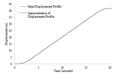
Figure 8: Ideal vs. Approximated Displacement Profiles of a Single Up Trip
A data set containing multiple trips is simply a series of linked single trips. To carry out multiple trip analysis, single trip analysis is looped until the end of the data set is reached. Since the software is capable of outputting the final displacement of each single trip, these can be stored allowing a spatial plot of the lift’s motion to be plotted over time. At this point, it is possible to begin to see the effects of accelerometer drift as the approximated positions can be compared to building data.
2.4 Processing Real Data
The introduction of real data introduced a series of issues to be tackled. The solution to each identified issue was integrated into the existing software such that it was capable of correctly representing the raw data.
2.5 Time Section Representation
Existing ideal lift kinematics curves are defined by a set of equations which are divided into time sections, identified by a change in jerk. To tackle an issue introduced with real data, a similar approach was taken. Rather than plotting continuous lines, five significant points are identified for each phase with respect to changes in acceleration, shown in Figure 9. A benefit of recording significant points rather than continuous data is the reduction in file size.

Figure 9: Representation of Time Sections For an Acceleration Phase
2.6 Spatial Plot Generation
The software creates two spatial plots; approximated and calibrated. The approximated spatial plot combines the displacement values stored for each single trip and adjusts the values at points where it is assumed that identical floors have been met. Access to real floor positions from building data allows the calibrated spatial plot to be generated. The approximated spatial plot is adjusted to the correct floor positions such that it can correctly plot the lift motion by floor and time of day.
3 Results
The first set of results processed were from data collected in a high-rise building in Central London, with an express zone using an accelerometer included in a low-cost consumer tablet. The existence of an express zone in the high-rise building resulted in the inability to generate a calibrated spatial plot due to the lack of accelerometer precision. The analysis was repeated using data collected in a low-rise office building. This three-story building does not have an express zone and therefore it is possible to calibrate and test the results to determine the accuracy of the software approximation.
3.1 High Rise Building
Figure 10 plots the raw displacement data against the approximated spatial plot generated by the software for the 39 floor building. The effects of drift are clear, and it is visible how the software has managed to tackle this problem.
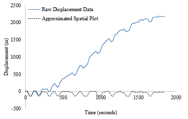
Figure 10: Calibrated vs. Approximated Displacement Profiles (High Rise Building)
3.2 Low Rise Building
Figure 11 plots the raw displacement profile without correction against the approximated spatial plot created by the software. It is clear from the scale of the raw data the significance of drift when modelling continuous lift motion.
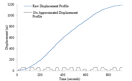
Figure 11: Calibrated vs. Approximated Displacement Profiles (Low Rise Building)
The lack of express zone in the low rise building allowed calibration to be carried out against real building data. Figure 12 plots the approximated spatial plot generated by the software against the adjusted spatial plot once calibration has been carried out.
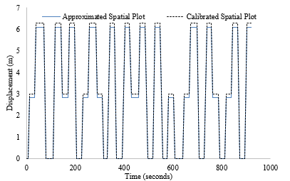
Figure 12: Approximated vs. Calibrated Displacement Profiles (Low Rise Building)
Table 1 shows a comparison between the approximated floor positions found by the software and the real floor positions provided from building data.
| Level 1 | Level 2 | Level 3 | |
| Approximated Floor Position | 0.00 | 2.83 | 6.08 |
| Real Floor Position | 0.00 | 3.00 | 6.29 |
| % Error | 0.00% | 5.61% | 3.38% |
Table 1: Comparison of Approximated and Real Floor Positions
4 Discussion and conclusions
Sensors are not ideal and solving a task with idealised data does not necessarily provide a real-world solution.
The high-rise data was collected by an accelerometer integrated in a budget tablet. The sampling frequency was inconsistent over the data set and the data contained significant noise. This made it particularly challenging to process, but ultimately led to a more robust software processing technique.
Using the accelerometer provided with an existing lift performance measurement tool [7] on a low-rise building, the floor positions were identified reliably with a floor position error of up to 5.6%. Given that in a commercial building, the floor to floor height is at least three meters, these errors do not inhibit the floor positions being identified. However, in the instance of a 100-meter express zone, a 5.6% error corresponds to 5.6 meters which is greater than a typical floor height. A more accurate sensor would be required to address this issue.
The software can be applied in lift monitoring applications, and the development of mathematical models to extrapolate passenger demand from stops [3]. It could be extended to work in three dimensions to be applied to other positioning monitoring applications.
There is a relationship between noise and sampling frequency, i.e. it is possible to reduce noise level by lowering the sampling frequency [8]. An investigation into the optimal sampling frequency and minimum resolution in relation to this application would be worthwhile. That is to minimise noise without compromising the identification of the key phases of the acceleration profile.
REFERENCES
- CIBSE, CIBSE Guide D: Transportation systems in buildings. Chartered Institution of Building Services Engineers London, 2015.
- L. Al-Sharif, ‘New Concepts in Lift Traffic Analysis: The Inverse S-P (I-S-P) Method’, in Proceedings of the International Conference of Elevator Technology, Amsterdam, 1992.
- R. D. Peters, ‘Lift Passenger Traffic Patterns: Applications, Current Knowledge and Measurement’. [Online]. Available: https://www.peters-research.com/index.php/support/articles-and-papers/50-lift-passenger-traffic-patterns-applications-current-knowledge-and-measurement. [Accessed: 22-Mar-2019].
- R. Basagoiti, M. Beamurgia, R. D. Peters, and S. Kaczmarczyk, ‘Origin Destination Matrix Estimation and Prediction in Vertical Transportation’, in Proceedings of The 2nd Symposium on Lift & Escalator Technology (CIBSE Lifts Group and The University of Northampton), 2012.
- R. D. Peters, ‘Ideal Lift Kinematics’. [Online]. Available: https://www.peters-research.com/index.php/support/articles-and-papers/53-ideal-lift-kinematics. [Accessed: 22-Mar-2019].
- R. M. Asha, M. D. Kavana, S. J. Parvathy, and C. M. Shreelakshmi, ‘Object-Oriented Programming and its Concepts’, IJSRD – Int. J. Sci. Res. Dev., vol. 5, no. 09, 2017.
- Peters Research, ‘Elevate Perform’, 2018. [Online]. Available: https://www.peters-research.com/. [Accessed: 26-Mar-2019].
- ‘RMS noise of accelerometers and gyroscopes’, Knowledge Base. [Online]. Available: http://base.xsens.com/hc/en-us/articles/115000224125-RMS-noise-of-accelerometers-and-gyroscopes. [Accessed: 28-Apr-2019].
BIOGRAPHICAL DETAILS
Anna Peters is a Research Assistant at Peters Research Ltd and a fourth-year engineering student studying for a MEng in Aeronautics and Astronautics at the University of Southampton. This paper is a shortened form of her third-year dissertation, supported by Professor Alexander I J Forrester (academic supervisor).
Richard Peters has a degree in Electrical Engineering and a Doctorate for research in Vertical Transportation. He is a director of Peters Research Ltd and a Visiting Professor at the University of Northampton. He has been awarded Fellowship of the Institution of Engineering and Technology, and of the Chartered Institution of Building Services Engineers. Dr Peters is the author of Elevate, elevator traffic analysis and simulation software.